Collider

Collider#

A collider is a variable that is influenced by two other variables of interest, creating a spurious association between them when we condition on (select or control for) the collider in our analysis.

Graphical Summary#

Fig

Key Formula#

The key formula for the concept of a collider is represented in a causal diagram as:

\[ X \rightarrow W \leftarrow Y \]

Where:

\(W\) is the collider variable
\(X\) is one cause of the collider
\(Y\) is another cause of the collider
The arrows (\(\rightarrow\)) indicate the direction of causal influence

This diagram illustrates that a collider (\(W\)) is a variable that is caused by both the exposure (\(X\)) and the outcome (\(Y\)), creating a situation where \(X\) and \(Y\) both flow into \(W\).

When we condition on (adjust for, stratify by, or select based on) a collider, we can induce a spurious association between its causes, even if they were originally independent.

Technical Details#

What Happens When We Control for Colliders#

When a collider is present and incorrectly controlled for:

\[ \text{Observed Association} = \text{True Effect} + \text{Collider Bias} \]

True Effect: The real biological relationship (may be zero)
Collider Bias: The false association created by conditioning on the collider
Observed Association: What we measure after incorrectly adjusting (often misleading!)

The Problem: Conditioning on Colliders Creates Bias#

Unlike confounders, colliders should NOT be included in regression models. Including a collider as a covariate can create spurious associations:

\[ Y = \beta_0 + \beta_1 X + \beta_2 \text{Collider} + \epsilon \quad \text{(WRONG!)} \]

This regression will give a biased estimate of \(\beta_1\) even when the true effect is zero.

Why This Happens: Selection Bias#

Controlling for a collider creates selection bias by conditioning on a variable that depends on both exposure and outcome:

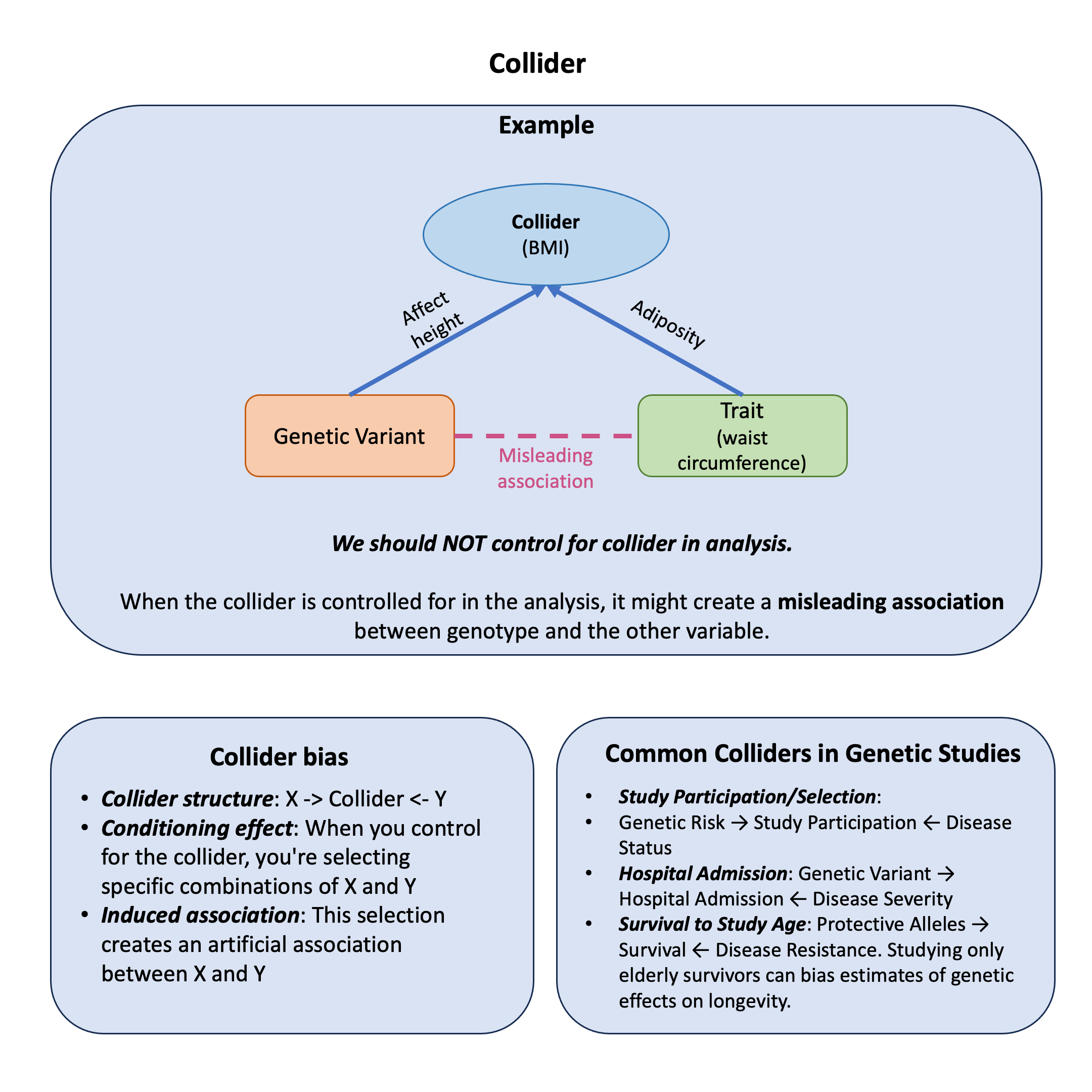
Collider structure: \(X \rightarrow \text{Collider} \leftarrow Y\)
Conditioning effect: When you control for the collider, you’re selecting specific combinations of X and Y
Induced association: This selection creates an artificial association between X and Y

Common Colliders in Genetic Studies#

Study Participation/Selection: Genetic Risk \(\leftarrow\) Study Participation \(\rightarrow\) Disease Status
Hospital Admission: Genetic Variant \(\leftarrow\) Hospital Admission \(\rightarrow\) Disease Severity
Survival to Study Age: Protective Alleles \(\leftarrow\) Survival \(\rightarrow\) Disease Resistance. Studying only elderly survivors can bias estimates of genetic effects on longevity.

The Key Principle#

Confounders: Control to remove bias
Colliders: Don’t control to avoid creating bias

Example#

Imagine you’re studying the relationship between genetic variants and waist circumference. You might think: “Since body mass index (BMI) is related to both genetics and body measurements, I should control for it to get a cleaner analysis, right?”

Wrong! This intuitive approach can actually create false associations where none exist.

Here’s the puzzle: What happens when we study the relationship between genetic variants and waist circumference, with and without “controlling” for BMI? You might expect that adding more variables to your model would make your analysis more accurate, but sometimes it can completely mislead you.

We’ll explore this using a simple simulation where we know the true relationships: imagine that a genetic variant affects height, therefore affecting BMI, but not affects waist circumference (WC) directly. However, BMI can also be affected by WC because of adiposity. So in this diagram BMI serves as the collider.

We’ll see how our results change when we don’t adjust for BMI versus when we mistakenly include it as a covariate.

Let’s create a scenario where we know the true relationships. We’ll generate data for 500 people with a genetic variant that affects height (and therefore BMI), plus waist circumference that’s completely independent of genetics.

rm(list=ls())
set.seed(15)

# Sample size
N <- 500

# Generate SNP (0, 1, 2 copies of height-increasing allele)
snp <- sample(0:2, N, replace = TRUE, prob = c(0.25, 0.5, 0.25))

# Generate waist circumference (completely independent of SNP)
# This represents individual differences in adiposity
waist_circumference <- rnorm(N, mean = 85, sd = 12)

Now we build the causal relationships that make BMI a collider:

# SNP affects height (each copy adds ~3cm)
height_cm <- 165 + 3 * snp + rnorm(N, 0, 6)

# Weight comes from two sources:
# 1. Height contributes through lean body mass
# 2. Waist circumference contributes through adiposity
weight_from_height <- 1 * height_cm  # Lean mass component
weight_from_adiposity <- 1.2 * waist_circumference  # Fat mass component
weight_kg <- weight_from_height + weight_from_adiposity - 140 + rnorm(N, 0, 5)

# Calculate BMI (the collider!)
bmi <- weight_kg / (height_cm/100)^2

Based on how the waist circumference is generated, it is independent from the genetic effect. Thus we should expect no signals when we test for the associations between waist circumference and SNPs. So we perform two analysis here:

ignore the collider (BMI), regress waist circumference on SNPs
consider the collider (BMI), regress waist circumference on SNPs and BMI

# Standardize variables for easier interpretation
snp_scaled <- scale(snp)[,1]
wc_scaled <- scale(waist_circumference)[,1]
bmi_scaled <- scale(bmi)[,1]

# Analysis 1: CORRECT - Don't adjust for BMI
correct_model <- lm(wc_scaled ~ snp_scaled)
correct_summary <- summary(correct_model)

# Analysis 2: INCORRECT - Adjust for BMI (the collider)
biased_model <- lm(wc_scaled ~ snp_scaled + bmi_scaled)
biased_summary <- summary(biased_model)

# Extract results
results <- data.frame(
  Analysis = c("Correct (no BMI)", "Incorrect (with BMI)"),
  Beta = c(
    round(correct_summary$coefficients[2, 1], 4),
    round(biased_summary$coefficients[2, 1], 4)
  ),
  SE = c(
    round(correct_summary$coefficients[2, 2], 4),
    round(biased_summary$coefficients[2, 2], 4)
  ),
  P_value = c(
    round(correct_summary$coefficients[2, 4], 4),
    round(biased_summary$coefficients[2, 4], 4)
  ),
  Significant = c(
    ifelse(correct_summary$coefficients[2, 4] < 0.05, "Yes", "No"),
    ifelse(biased_summary$coefficients[2, 4] < 0.05, "Yes", "No")
  )
)

Let’s taka a look at the results:

results

A data.frame: 2 x 5
Analysis	Beta	SE	P_value	Significant
<chr>	<dbl>	<dbl>	<dbl>	<chr>
Correct (no BMI)	-0.0044	0.0448	0.9218	No
Incorrect (with BMI)	0.0715	0.0183	0.0001	Yes

This example shows how controlling for BMI creates a false association between a genetic variant and waist circumference, even though no true biological relationship exists. The “controlling for everything” approach that seems so intuitive actually generates bias.

The key lesson: Before adjusting for any variable, ask whether it could be caused by both your exposure and outcome. If yes, conditioning on it may introduce collider bias rather than remove confounding.

In real studies, this type of bias could lead to false discoveries, wasted resources chasing non-existent mechanisms, and potentially harmful clinical recommendations based on spurious associations.