Genetic Relationship Matrix#
Genetic relationship matrix (GRM) captures how related individuals are to each other at the genomic level by measuring the proportion of shared genetic variants across their genomes, and quantifies the genetic similarity between every pair of individuals in the population.
Graphical Summary#
Key Formula#
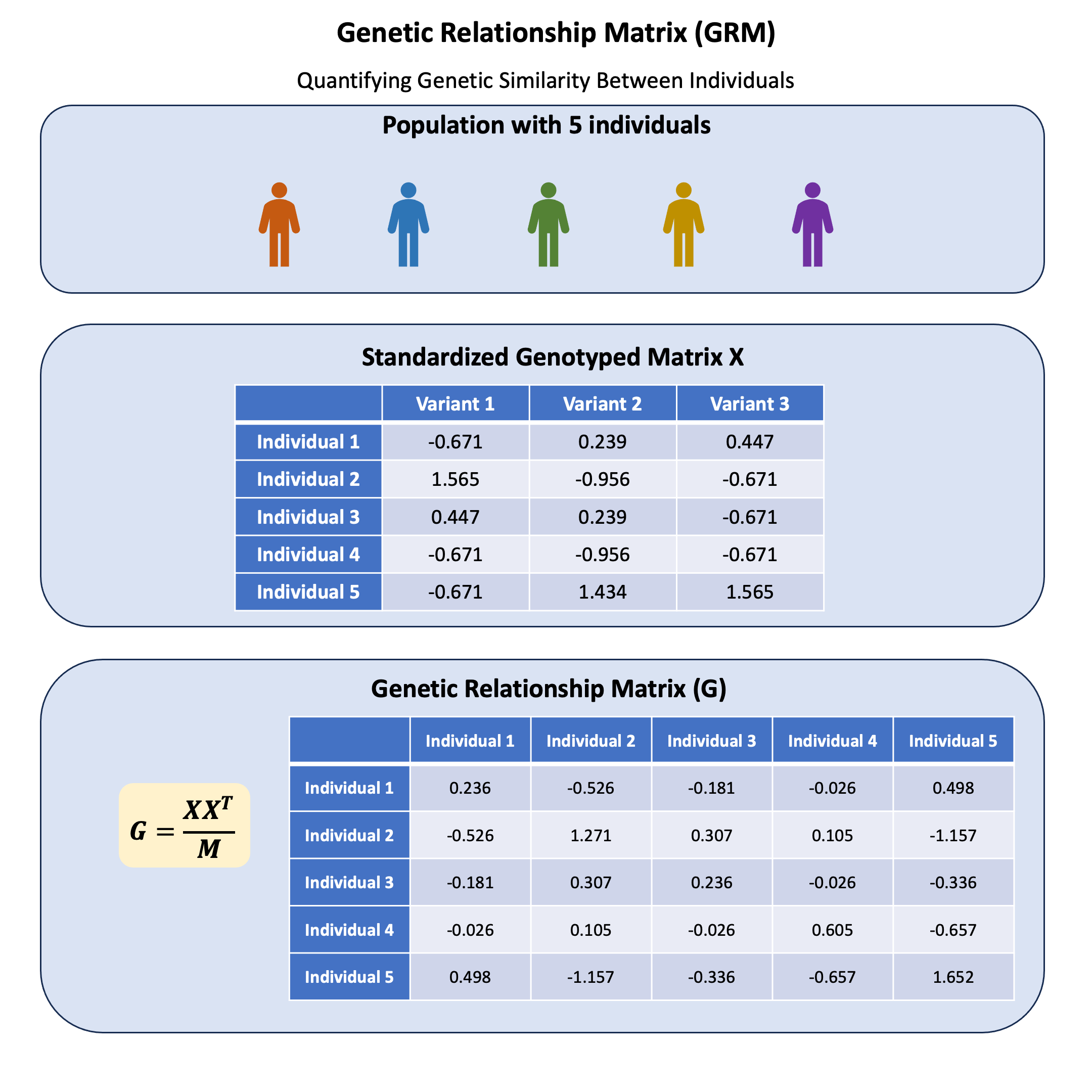
Genomic Relationship Matrix (GRM) is a standardized version of the kinship matrix that accounts for allele frequencies. One common formulation is:
Where:
\(\mathbf{X}\) is the scaled genotype matrix of \(N\) individuals and \(M\) genetic variants.
\( \mathbf{G} \) is an \( N \times N \) matrix capturing the pairwise genetic relationships.
Technical Details#
Relationship to Kinship#
What is kinship? Kinship measures how much DNA two people share from common ancestors. You share about 50% of your DNA with each parent. If you and your cousin both have the same grandparents, you share about 12.5% of your DNA with him or her. Strangers typically share almost no DNA.
So what’s different about the GRM? Instead of relying on family trees, the GRM looks directly at thousands of genetic variants and asks: “Based on what I can actually observe in the DNA, how similar are these two people?”
What’s this about allele frequencies? Here’s the key insight: if everyone in your population has allele A at some position, then you and I both having A tells us nothing special. But if only 2% of people have allele B, and we both have it, that’s much more informative about our relatedness. The GRM weights rare shared alleles more heavily than common ones.
Why is this better for statistical genetics? Kinship coefficients measure the probability that two individuals share alleles identical by descent (IBD) - alleles inherited from a recent common ancestor. The GRM, in contrast, measures actual allele sharing across the genome regardless of recent ancestry. This means the GRM captures both familial relationships and population structure, making it more comprehensive for statistical genetics applications where we want to account for all sources of genetic similarity.
Scaling Properties#
Because \(\mathbf{X}\) is standardized across individuals (each variant has variance = 1), the diagonal elements of \(\mathbf{G}\) aren’t necessarily 1. The diagonal tells you how “typical” each individual is compared to the population average.
Example#
We’ve been working with the same 5 individuals and 3 genetic variants throughout our examples so far. Now let’s see what happens when we use this data to compute a GRM. Which individuals appear most genetically similar to each other? Do any of them look like they might be related? And what do the numbers in the GRM actually tell us about genetic relationships?
Let’s calculate the GRM step by step and interpret what each element means in terms of genetic similarity.
# Clear the environment
rm(list = ls())

# Define genotypes for 5 individuals at 3 variants
# These represent actual alleles at each position
# For example, Individual 1 has genotypes: CC, CT, AT
genotypes <- c(
 "CC", "CT", "AT",  # Individual 1
 "TT", "TT", "AA",  # Individual 2
 "CT", "CT", "AA",  # Individual 3
 "CC", "TT", "AA",  # Individual 4
 "CC", "CC", "TT"   # Individual 5
)
# Reshape into a matrix
N = 5
M = 3
geno_matrix <- matrix(genotypes, nrow = N, ncol = M, byrow = TRUE)
rownames(geno_matrix) <- paste("Individual", 1:N)
colnames(geno_matrix) <- paste("Variant", 1:M)

alt_alleles <- c("T", "C", "T")

# Convert to raw genotype matrix using the additive / dominant / recessive model
Xraw_additive <- matrix(0, nrow = N, ncol = M) # dount number of non-reference alleles

rownames(Xraw_additive) <- rownames(geno_matrix)
colnames(Xraw_additive) <- colnames(geno_matrix)

for (i in 1:N) {
  for (j in 1:M) {
    alleles <- strsplit(geno_matrix[i,j], "")[[1]]
    Xraw_additive[i,j] <- sum(alleles == alt_alleles[j])
  }
}

X <- scale(Xraw_additive, center = TRUE, scale = TRUE)
The scaled genotype matrix X (scaled with respective for column) is:
X
| Variant 1 | Variant 2 | Variant 3 | |
|---|---|---|---|
| Individual 1 | -0.6708204 | 0.2390457 | 0.4472136 |
| Individual 2 | 1.5652476 | -0.9561829 | -0.6708204 |
| Individual 3 | 0.4472136 | 0.2390457 | -0.6708204 |
| Individual 4 | -0.6708204 | -0.9561829 | -0.6708204 |
| Individual 5 | -0.6708204 | 1.4342743 | 1.5652476 |
The GRM can be calculated as:
# calculate the GRM
GRM = (X %*% t(X)) / M
GRM
| Individual 1 | Individual 2 | Individual 3 | Individual 4 | Individual 5 | |
|---|---|---|---|---|---|
| Individual 1 | 0.23571429 | -0.5261905 | -0.18095238 | -0.02619048 | 0.4976190 |
| Individual 2 | -0.52619048 | 1.2714286 | 0.30714286 | 0.10476190 | -1.1571429 |
| Individual 3 | -0.18095238 | 0.3071429 | 0.23571429 | -0.02619048 | -0.3357143 |
| Individual 4 | -0.02619048 | 0.1047619 | -0.02619048 | 0.60476190 | -0.6571429 |
| Individual 5 | 0.49761905 | -1.1571429 | -0.33571429 | -0.65714286 | 1.6523810 |