Proportion of Variance Explained and Heritability#
Proportion of variance explained (PVE) measures how much of the total variation in a trait (like height or disease risk) can be attributed to specific variables in your statistical model (e.g., genetic variants). Heritability is a specific application of this concept that measures how much of the variation in a trait across a population can be explained by genetic differences.
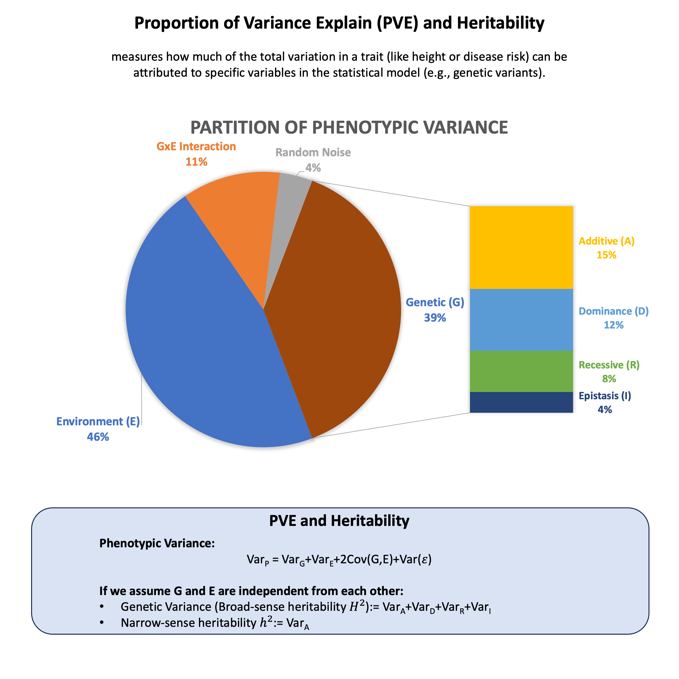
Graphical Summary#
Key Formula#
Any phenotype can be modeled as the sum of genetic and environmental effects, i.e., \(\text{Phenotype}~(Y) = \text{Genotype}~(G) + \text{Environment}~(E)\), and under the assumption that G and E are independent from each other, the proportion of variance explained (PVE) by genetic effect alone (also called broad-sense heritability \(H^2\)) can be derived as
where:
\(\text{Var}_G\) is the genetic variance component
\(\text{Var}_E\) is the environmental variance component
Technical Details#
Components of Variance#
Any phenotype can be modeled as the sum of genetic and environmental effects:
The phenotypic variance in the trait can then be partitioned as:
Where:
\(\text{Var}_G\) is the genetic variance component
\(\text{Var}_E\) is the environmental variance component
\(\text{Cov}(G,E)\) is the covariance between genetic and environmental effects
Broad-sense Heritability#
In controlled experimental settings, we can design studies where \(\text{Cov}(G,E)\) is minimized and effectively set to zero. In such cases, heritability is defined as the proportion of phenotypic variance attributable to all genetic effects:
This represents the proportion of phenotypic variance attributable to genetic variance.
Narrow-sense Heritability#
Narrow-sense heritability (\(h^2\)): The proportion attributable to only additive genetic effects:
Where \(\text{Var}_A\) is the additive genetic variance, a component of \(\text{Var}_G\).
Other components of \(\text{Var}_G\) includes \(\text{Var}_D\) (dominance variance) and \(\text{Var}_I\) (epistatic variance, i.e., gene-gene interaction)
Example#
When we say a trait has “50% heritability,” what does that actually mean? Let’s explore this using a simple example with 5 individuals and see how much of their trait variation comes from genetics versus other factors.
Imagine we’re studying a trait in 5 people, and we know their genotypes at 3 genetic variants. Each person has different combinations of alleles - some have more “risk” alleles than others. The key question is: How much of the differences we see in their trait values can be explained by their genetic differences?
We’ll calculate this step by step, first using a scenario where each person has their own unique genetic effect, then comparing it to a simpler case where the genetic variant has the same effect size for everyone. This will help us understand what “proportion of variance explained” really means in practice.
# Clear the environment
rm(list = ls())
set.seed(11)
# Define genotypes for 5 individuals at 3 variants
# These represent actual alleles at each position
# For example, Individual 1 has genotypes: CC, CT, AT
genotypes <- c(
 "CC", "CT", "AT",  # Individual 1
 "TT", "TT", "AA",  # Individual 2
 "CT", "CT", "AA",  # Individual 3
 "CC", "TT", "AA",  # Individual 4
 "CC", "CC", "TT"   # Individual 5
)
# Reshape into a matrix
N = 5
M = 3
geno_matrix <- matrix(genotypes, nrow = N, ncol = M, byrow = TRUE)
rownames(geno_matrix) <- paste("Individual", 1:N)
colnames(geno_matrix) <- paste("Variant", 1:M)

alt_alleles <- c("T", "C", "T")

# Convert to raw genotype matrix using the additive / dominant / recessive model
Xraw_additive <- matrix(0, nrow = N, ncol = M) # dount number of non-reference alleles

rownames(Xraw_additive) <- rownames(geno_matrix)
colnames(Xraw_additive) <- colnames(geno_matrix)

for (i in 1:N) {
  for (j in 1:M) {
    alleles <- strsplit(geno_matrix[i,j], "")[[1]]
    Xraw_additive[i,j] <- sum(alleles == alt_alleles[j])
  }
}

X <- scale(Xraw_additive, center = TRUE, scale = TRUE)
Random effect#
Following the example in Lecture: random effect, we then calculate the PVE of the variants.
beta <- rnorm(N, mean = 0, sd = 1)
epsilon <- rnorm(N, mean = 0, sd = 0.3)
Y <- X[, 1] * beta + epsilon
beta
- -0.591031102584368
- 0.026594369016167
- -1.51655309708187
- -1.36265334929581
- 1.17848915603162
Now let’s calculate the PVE using the definition.
# Calculate PVE using the definition: PVE = Var(G) / Var(Y)
# where G = X * beta (genetic component)
G <- X[, 1] * beta
var_G <- var(G)
var_Y <- var(Y)
PVE <- var_G / var_Y
PVE
Fixed Effect#
As we discussed before, in the fixed effect model, the genetic effect \(\beta\) is a constant parameter that applies uniformly to all individuals. We then calculate the PVE of the variants.
# Fixed effect: single beta value for all individuals
beta <- 0.8  # Fixed effect size
epsilon <- rnorm(N, mean = 0, sd = 0.3)
Y <- X[, 1] * beta + epsilon
beta
Now let’s calculate the PVE using the definition as well:
# Calculate PVE using the definition: PVE = Var(G) / Var(Y)
# where G = X * beta (genetic component)
G <- X[, 1] * beta
var_G <- var(G)
var_Y <- var(Y)
PVE <- var_G / var_Y
PVE