Meta-Analysis Fixed Effect#
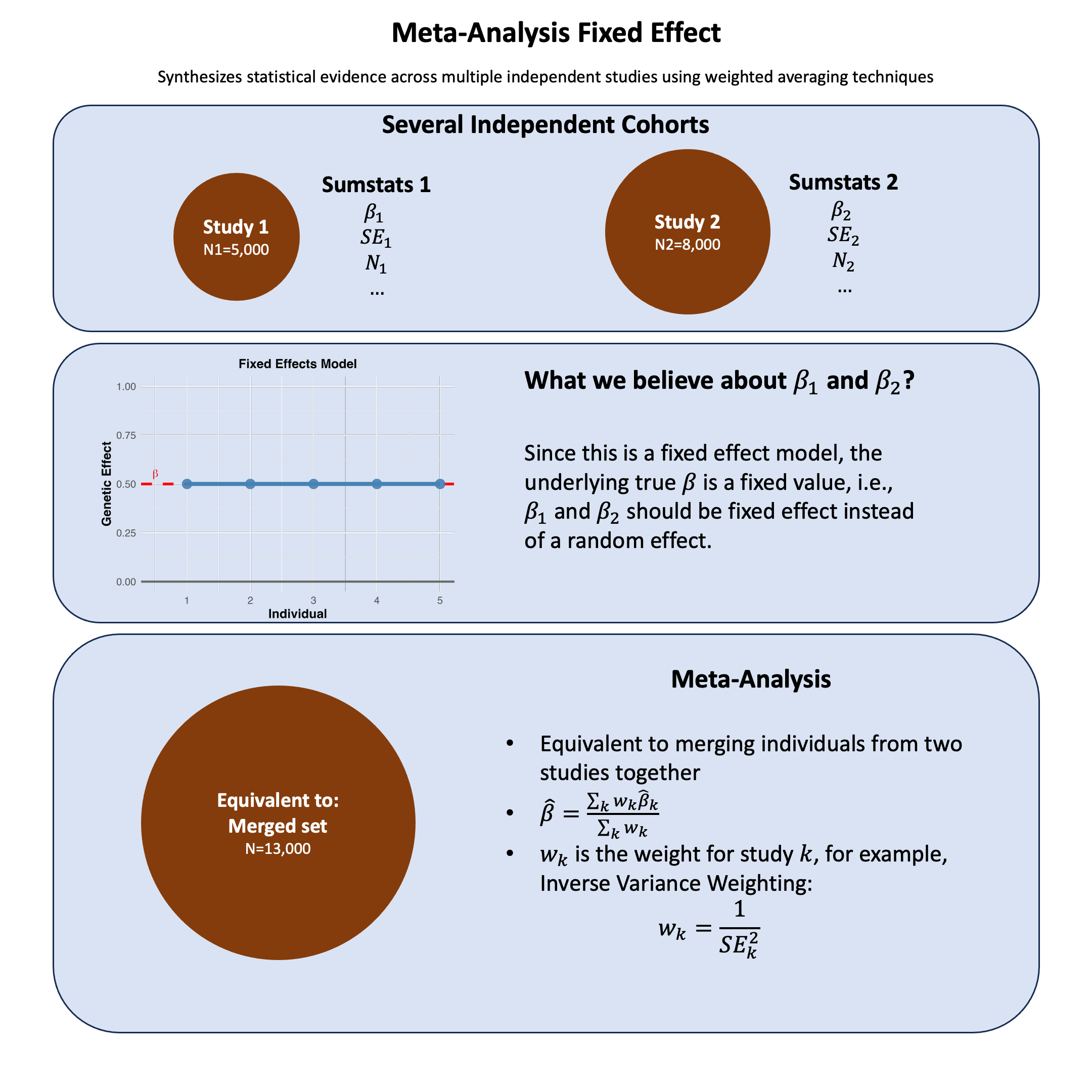
Fixed-effect meta-analysis combines study-specific estimates under the assumption of a common fixed true effect, making it mathematically equivalent to analyzing all individuals as if they came from a single pooled dataset.
Graphical Summary#
Key Formula#
In meta-analysis, the weighted mean effect size for a fixed-effects model is calculated as:
Where:
\(\hat{\beta}\) is the combined effect estimate across all studies
\(\hat{\beta}_i\) is the effect estimate from study \(k\)
\(w_k\) is the weight assigned to study \(k\)
\(K\) is the number of studies
Technical Details#
Why Do We Need Meta-Analysis?#
Individual studies have limitations:
Small sample sizes -> low statistical power
Population-specific effects -> limited generalizability
Random variation -> unreliable estimates
Meta-analysis provides:
Larger effective sample size -> higher power to detect true effects
More precise effect estimates -> narrower confidence intervals
Broader population representation -> better generalizability
How the Weighting Works#
The key insight is that not all studies should contribute equally. Studies with more information should have more influence on the final result.
Weight is based on precision:
Where \(\text{SE}_k\) is the standard error of study \(k\).
This means:
Large studies (small SE) get high weight: more influence
Small studies (large SE) get low weight: less influence
Precise studies contribute more to the final estimate
The Fixed-Effects Assumption#
Fixed-effects meta-analysis assumes that all studies estimate the same true effect. Any differences between studies are due to random sampling variation only.
When to use fixed-effects:
Studies are very similar (same populations, methods, designs)
Low heterogeneity between study results
Want to estimate the common effect size
When NOT to use fixed-effects:
Studies differ substantially in populations or methods
High heterogeneity between results
Different genetic architectures across populations
Important Limitations#
Garbage in, garbage out: Meta-analysis cannot fix poorly designed individual studies
Publication bias: Published studies may not represent all conducted research
Population differences: Genetic effects may genuinely differ across populations
Example#
This example demonstrates a meta-analysis of genetic variants across two European cohorts. We’ll analyze 3 genetic variants (SNPs) that have been genotyped in both cohorts and combine their effects using fixed-effects meta-analysis.
We first generate the summary statistics for 3 variants from two independent European cohorts with different sample sizes (N=8000 and N=5500), and assuming that they are from the same genetic ancestry so they can be meta-analyzed.
Then we perform fixed-effects meta-analysis combining results using:
Sample size weighting (weight proportional to \(\frac{1}{\sqrt{N}}\))
Inverse variance weighting (weight = \(\frac{1}{\text{SE}^2}\))
Lastly we plot the effect size and p-values for each variant and compare the results from separate cohorts and meta-analysis results. We also compare the variance based on the sample size and inverse variance.
rm(list=ls())
set.seed(17)

# 1. Simulate genotype data (0/1/2) for a single SNP
N1 <- 5000
N2 <- 8000
maf1 <- 0.3
maf2 <- 0.35

variant_pop1 <- rbinom(N1, 2, maf1)
variant_pop2 <- rbinom(N2, 2, maf2)
# 2. Simulate phenotype with fixed effect beta=1 and noise
beta <- 1
y_pop1 <- beta * variant_pop1 + rnorm(N1, 0, 3)
y_pop2 <- beta * variant_pop2 + rnorm(N2, 0, 3)
# 3. Run regression in each population
lm_pop1 <- lm(y_pop1 ~ variant_pop1)
lm_pop2 <- lm(y_pop2 ~ variant_pop2)

# Extract summary statistics
beta_pop1 <- coef(lm_pop1)["variant_pop1"]
se_pop1 <- summary(lm_pop1)$coefficients["variant_pop1", "Std. Error"]

beta_pop2 <- coef(lm_pop2)["variant_pop2"]
se_pop2 <- summary(lm_pop2)$coefficients["variant_pop2", "Std. Error"]
# 4. Fixed-effect meta-analysis
w1 <- 1 / se_pop1^2
w2 <- 1 / se_pop2^2

beta_meta <- (beta_pop1 * w1 + beta_pop2 * w2) / (w1 + w2)
se_meta <- sqrt(1 / (w1 + w2))
z_meta <- beta_meta / se_meta
p_meta <- 2 * pnorm(-abs(z_meta))
res_meta = data.frame(beta_meta, se_meta, z_meta, p_meta)
rownames(res_meta) = NULL
res_meta
| beta_meta | se_meta | z_meta | p_meta |
|---|---|---|---|
| <dbl> | <dbl> | <dbl> | <dbl> |
| 1.015251 | 0.04011815 | 25.30654 | 2.706622e-141 |
Alternatively we can simply combine all individuals into one and calculate the summary statistics for this variant.
# 5. Pooled analysis
variant_all <- c(variant_pop1, variant_pop2)
y_all <- c(y_pop1, y_pop2)

lm_all <- lm(y_all ~ variant_all)
beta_all <- coef(lm_all)["variant_all"]
se_all <- summary(lm_all)$coefficients["variant_all", "Std. Error"]
z_all <- beta_all / se_all
p_all <- 2 * pnorm(-abs(z_all))
res_merged = data.frame(beta_all, se_all, z_all, p_all)
rownames(res_merged) = NULL
res_merged
| beta_all | se_all | z_all | p_all |
|---|---|---|---|
| <dbl> | <dbl> | <dbl> | <dbl> |
| 1.013051 | 0.03998501 | 25.33578 | 1.289396e-141 |
# 6. Compare results

res_meta
res_merged
| beta_meta | se_meta | z_meta | p_meta |
|---|---|---|---|
| <dbl> | <dbl> | <dbl> | <dbl> |
| 1.015251 | 0.04011815 | 25.30654 | 2.706622e-141 |
| beta_all | se_all | z_all | p_all |
|---|---|---|---|
| <dbl> | <dbl> | <dbl> | <dbl> |
| 1.013051 | 0.03998501 | 25.33578 | 1.289396e-141 |
The results are almost identical (after numerical rounding).