Linear Mixed Model#
When we want to study a specific genetic variant as a fixed effect but know there are countless unmeasured factors affecting our trait, linear mixed models offer a practical solution: use a random effect based on genetic similarity to absorb all that unmeasured heterogeneity.
Graphical Summary#
Key Formula#
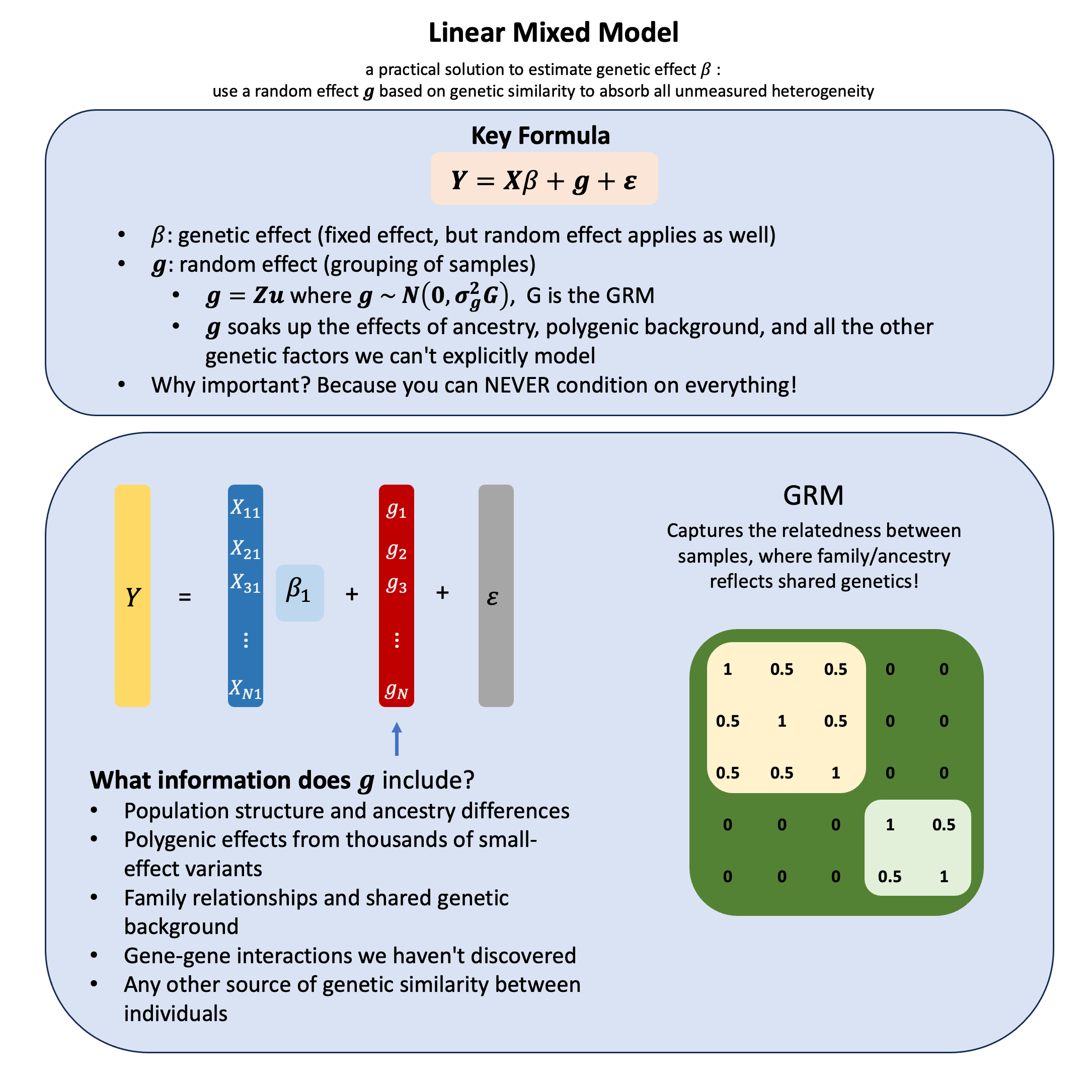
In the linear mixed model (mixed because it incorporate both the fixed and the random effects), which accurately represent non-independent data structures for a variant,
where:
\(\mathbf{Y}\) is the \(N \times 1\) vector of phenotypes
\(\mathbf{X}\) is the \(N \times 1\) design matrix for fixed effects (e.g., the specific genetic variant we’re testing, plus measurable covariates like age and sex)
\(\beta\) is the scalar of fixed genetic effect coefficient (unknown, to be estimated)
\(\mathbf{g}\) is the \(N \times 1\) vector of random effects that captures all the genetic factors we can’t or don’t want to model explicitly - population structure, polygenic background, family relationships, and countless unknown genetic influences
\(\boldsymbol{\epsilon}\) is the \(N \times 1\) vector of residual errors, where \(\boldsymbol{\epsilon} \sim N(0, \sigma^2_e\mathbf{I})\)
Technical Details#
Random Effects Decomposition: \(\mathbf{g}\) and \(\mathbf{Zu}\)#
The key insight is that for a genetic variant, there are countless things to account for: age, sex, ancestry, thousands of genes and unknown ones. We can never write the complete model:
Instead, we approximate it as:
where \(\mathbf{g}\) soaks up the effects of ancestry, polygenic background, and all the other genetic factors we can’t explicitly model. It’s not as precise as conditioning on everything, but it’s the best we can do when complete conditioning is impossible.
What information should \(\mathbf{g}\) capture? Ideally, \(\mathbf{g}\) should include:
Population structure and ancestry differences
Polygenic effects from thousands of small-effect variants
Family relationships and shared genetic background
Gene-gene interactions we haven’t discovered
Any other source of genetic similarity between individuals
The random effects term g can be decomposed as:
where:
\(\mathbf{g}\) is the \(N \times 1\) vector of random effects for \(N\) individuals, where \(\mathbf{g} \sim N(\mathbf{0}, \sigma^2_g\mathbf{G})\)
\(\mathbf{G}\) is the genetic relationship matrix (GRM) that measures genetic similarity between individuals, effectively capturing all the unmeasured genetic factors through genome-wide similarity patterns
\(\mathbf{Z}\) is the \(N \times M\) genotype matrix for \(M\) genetic variants
\(\mathbf{u} \sim N(0, \sigma_u^2\mathbf{I})\) is a \(M \times 1\) vector of random SNP effects
Formally known as the infinitesmal model
Popular LMM Methods in Statistical Genetics#
Method |
Purpose |
Key Innovation |
Scale/Application |
|---|---|---|---|
GCTA |
Heritability estimation and association testing |
Uses genome-wide SNPs to construct genetic relationship matrix (GRM) |
\(h^2 = \frac{\sigma^2_u}{\sigma^2_u + \sigma^2_e}\) estimation |
GEMMA |
Fast genome-wide association studies with population structure control |
Efficient algorithms for large-scale GWAS with kinship correction |
Computationally efficient for large-scale data |
BOLT-LMM |
Ultra-fast mixed model association testing |
Bayesian sparse linear mixed model approach |
Hundreds of thousands of individuals |
SAIGE |
Association testing for binary and quantitative traits |
Handles unbalanced case-control studies efficiently |
Saddlepoint approximation for computational efficiency |
REGENIE |
Whole genome regression with prediction |
Two-step procedure combining whole-genome regression to solve mixed models |
Use ridge regression instead of conventional LMM |
Example#
What happens when we acknowledge that our trait is influenced not just by one specific variant, but also by a “genetic background” from all the other variants we’re not explicitly testing? Let’s see how linear mixed models capture this reality.
We’ll use the same 5 individuals, but now we’ll model two sources of genetic influence: a fixed effect from one specific variant we’re studying, plus a random polygenic effect that represents the combined influence of all variants acting as genetic background. How much does each component contribute to the total genetic influence on our trait?
# Clear the environment
rm(list = ls())
set.seed(13)
library(MASS) # For mvrnorm function
# Define genotypes for 5 individuals at 3 variants
# These represent actual alleles at each position
# For example, Individual 1 has genotypes: CC, CT, AT
genotypes <- c(
 "CC", "CT", "AT",  # Individual 1
 "TT", "TT", "AA",  # Individual 2
 "CT", "CT", "AA",  # Individual 3
 "CC", "TT", "AA",  # Individual 4
 "CC", "CC", "TT"   # Individual 5
)

# Reshape into a matrix
N = 5
M = 3
geno_matrix <- matrix(genotypes, nrow = N, ncol = M, byrow = TRUE)
rownames(geno_matrix) <- paste("Individual", 1:N)
colnames(geno_matrix) <- paste("Variant", 1:M)

alt_alleles <- c("T", "C", "T")

# Convert to raw genotype matrix using the additive model
Xraw_additive <- matrix(0, nrow = N, ncol = M) # count number of non-reference alleles

rownames(Xraw_additive) <- rownames(geno_matrix)
colnames(Xraw_additive) <- colnames(geno_matrix)

for (i in 1:N) {
  for (j in 1:M) {
    alleles <- strsplit(geno_matrix[i,j], "")[[1]]
    Xraw_additive[i,j] <- sum(alleles == alt_alleles[j])
  }
}

X <- scale(Xraw_additive, center = TRUE, scale = TRUE)
We generate the data according to a linear mixed model:
# Linear Mixed Model: Y = X*beta + g + epsilon
# where g = Z*u represents random polygenic effects

# Fixed effect for variant 1
beta <- 0.8  # Fixed effect size for variant 1

# Create Genetic Relationship Matrix (GRM) using all variants
# GRM = (1/M) * X_raw * X_raw^T, where X_raw is the standardized genotype matrix
GRM <- (1/M) * X %*% t(X)
cat("Genetic Relationship Matrix (GRM):\n")
GRM

# Generate random polygenic effects: g ~ N(0, sigma_u^2 * GRM)
sigma_u <- 0.5  # Standard deviation of random effects
g <- mvrnorm(n = 1, mu = rep(0, N), Sigma = sigma_u^2 * GRM)
g <- as.vector(g)

# Residual errors
sigma_e <- 0.3  # Standard deviation of residual errors
epsilon <- rnorm(N, mean = 0, sd = sigma_e)

# Generate phenotype with both fixed and random effects
Y <- X[, 1] * beta + g + epsilon
Genetic Relationship Matrix (GRM):
| Individual 1 | Individual 2 | Individual 3 | Individual 4 | Individual 5 | |
|---|---|---|---|---|---|
| Individual 1 | 0.23571429 | -0.5261905 | -0.18095238 | -0.02619048 | 0.4976190 |
| Individual 2 | -0.52619048 | 1.2714286 | 0.30714286 | 0.10476190 | -1.1571429 |
| Individual 3 | -0.18095238 | 0.3071429 | 0.23571429 | -0.02619048 | -0.3357143 |
| Individual 4 | -0.02619048 | 0.1047619 | -0.02619048 | 0.60476190 | -0.6571429 |
| Individual 5 | 0.49761905 | -1.1571429 | -0.33571429 | -0.65714286 | 1.6523810 |
We can estimate the PVE again by each component:
# In LMM, total genetic variance = fixed effects variance + random effects variance
# Fixed genetic component from variant 1
G_fixed <- X[, 1] * beta

# Random genetic component (polygenic background)
G_random <- g

# Total genetic component
G_total <- G_fixed + G_random

# Calculate variance components
var_G_fixed <- var(G_fixed)
var_G_random <- var(G_random)
var_G_total <- var(G_total)
var_Y <- var(Y)

# PVE calculations
PVE_fixed <- var_G_fixed / var_Y           # PVE from fixed effects only
PVE_random <- var_G_random / var_Y         # PVE from random effects only
PVE_total <- var_G_total / var_Y           # Total PVE

cat("PVE Components:\n")
cat("PVE_fixed (variant 1) =", round(PVE_fixed, 4), "\n")
cat("PVE_random (polygenic) =", round(PVE_random, 4), "\n")
cat("PVE_total =", round(PVE_total, 4), "\n\n")
PVE Components:
PVE_fixed (variant 1) = 0.8187
PVE_random (polygenic) = 0.1212
PVE_total = 0.67
Note that the same framework applies when the genetic effect \(\beta\) is modeled as a random effect rather than fixed.