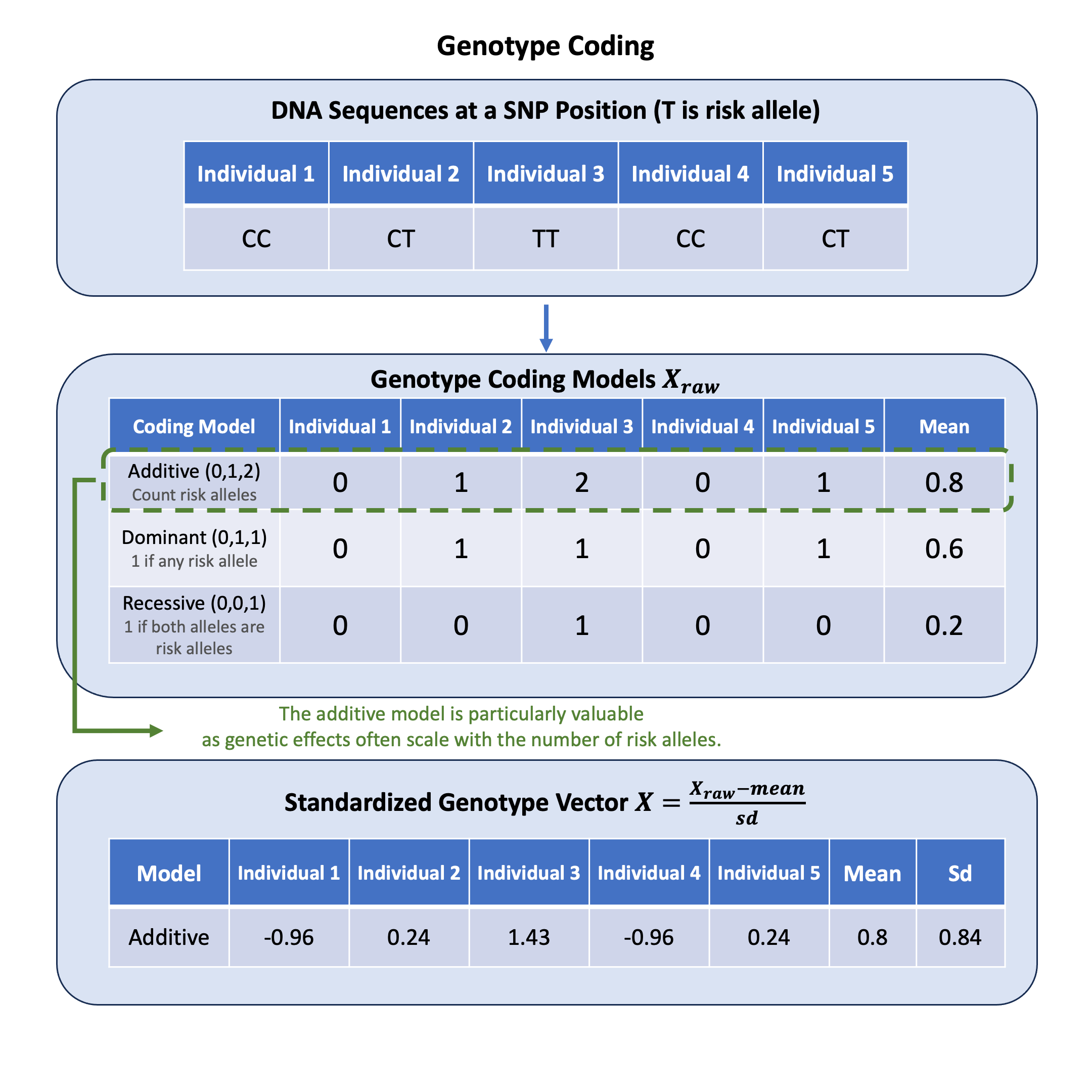
Genotype Coding#
Genotype coding converts DNA nucleotide pairs into numerical values for statistical analysis, with the additive model being particularly valuable because genetic effects often accumulate proportionally with each additional copy of a variant.
Graphical Summary#
Key Formula#
We use \(\mathbf{X}_\text{raw}\) to denote the raw genotype matrix (an \(N \times M\) matrix representing genotypes for \(N\) individuals at \(M\) variants). By default, we use the additive coding model which takes values from \(\{0, 1, 2\}\) representing the count of alternative alleles.
We use \(\mathbf{X}\) to denote the standardized genotype matrix, which is the normalized version of \(\mathbf{X}_\text{raw}\). Why standardization? Different genetic variants have different allele frequencies, leading to different variances in their raw genotype values. Without standardization, effect sizes \(\beta\) are not comparable across variants - a \(\beta = 0.1\) effect on a rare variant affects the population differently than the same effect on a common variant.
Standardization puts all variants on the same scale, making effect sizes directly comparable across variants. This is essential for analyses that combine information across multiple variants, as we will see in Lecture: proportion of variance explained, Lecture: random effect, Lecture: Bayesian normal mean model, etc.
For each column \(j\) (the \(j\)-th variant):
Where:
\(\mu_j = \frac{1}{N}\sum_{i=1}^{N} X_{\text{raw},ij}\) (mean of the \(j\)-th variant)
\(\sigma_j = \sqrt{\frac{1}{N-1}\sum_{i=1}^{N} (X_{\text{raw},ij} - \mu_j)^2}\) (standard deviation of the \(j\)-th variant)
Technical Details#
Coding Models#
For diploid organisms (with two copies of each chromosome, e.g., human), we can use different coding models:
Additive model (default): takes value from \(\{0, 1, 2\}\)
0: Homozygous for reference allele (AA)
1: Heterozygous (Aa)
2: Homozygous for alternative allele (aa)
Represents the count of alternative alleles
Dominant model: takes value from \(\{0, 1\}\)
0: Homozygous for reference allele (AA)
1: Either heterozygous or homozygous for alternative allele (Aa or aa)
Represents the presence of at least one copy of the alternative allele
Recessive model: takes value from \(\{0, 1\}\)
0: Either homozygous for reference allele or heterozygous (AA or Aa)
1: Homozygous for alternative allele (aa)
Represents when both copies of the alternative allele are present
Standardized Genotype Matrix#
\(\mathbf{X}\) is a normalized version of \(\mathbf{X}_\text{raw}\) where each variant is scaled to have mean 0 and variance 1.
For each column \(j\) (variant):
\(\mu_j = \frac{1}{N}\sum_{i=1}^{N} X_{\text{raw},ij}\) (mean of the \(j\)-th variant)
Represents the average number of alternative alleles at the \(j\)-th variant in the sample under the additive model
\(\sigma_j = \sqrt{\frac{1}{N-1}\sum_{i=1}^{N} (X_{\text{raw},ij} - \mu_j)^2}\) (standard deviation of the \(j\)-th variant)
Measures the variability in the number of alternative alleles at the \(j\)-th variant
This standardization ensures that:
Each column of \(\mathbf{X}\) has mean 0 and variance 1
The standardized values reflect the deviation from the population mean in units of standard deviation
All variants contribute equally to downstream statistical analyses regardless of their allele frequencies
Example#
Let’s say we have genetic data from 5 individuals tested at 3 different variants. How do we go from the actual genotype calls (like “CC” or “CT”) to the numerical matrices used in statistical genetics? What happens when we apply different coding models to the same data? And how do we standardize these matrices in R?
# Clear the environment
rm(list = ls())

# Define genotypes for 5 individuals at 3 variants
# These represent actual alleles at each position
# For example, Individual 1 the following nucleotides on three variants: CC, CT, AT
genotypes <- c(
 "CC", "CT", "AT",  # Individual 1
 "TT", "TT", "AA",  # Individual 2
 "CT", "CT", "AA",  # Individual 3
 "CC", "TT", "AA",  # Individual 4
 "CC", "CC", "TT"   # Individual 5
)
# Reshape into a matrix
N = 5
M = 3
geno_matrix <- matrix(genotypes, nrow = N, ncol = M, byrow = TRUE)
rownames(geno_matrix) <- paste("Individual", 1:N)
colnames(geno_matrix) <- paste("Variant", 1:M)
The raw genotype matrix is:
geno_matrix
| Variant 1 | Variant 2 | Variant 3 | |
|---|---|---|---|
| Individual 1 | CC | CT | AT |
| Individual 2 | TT | TT | AA |
| Individual 3 | CT | CT | AA |
| Individual 4 | CC | TT | AA |
| Individual 5 | CC | CC | TT |
Then we assign the alternative allele for each variant:
# Define alternative alleles for each variant
alt_alleles <- c("T", "C", "T")
names(alt_alleles) <- colnames(geno_matrix)
Now let’s convert the variants information for the individuals into a raw genotype matrix, under three different models:
# Convert to raw genotype matrix using the additive / dominant / recessive model
Xraw_additive <- matrix(0, nrow=nrow(geno_matrix), ncol=ncol(geno_matrix)) # count number of non-reference alleles
Xraw_dominant <- matrix(0, nrow=nrow(geno_matrix), ncol=ncol(geno_matrix)) # presence of alternative allele
Xraw_recessive <- matrix(0, nrow=nrow(geno_matrix), ncol=ncol(geno_matrix)) # two copies of alternative allele required

rownames(Xraw_additive) <- rownames(Xraw_dominant) <- rownames(Xraw_recessive) <- rownames(geno_matrix)
colnames(Xraw_additive) <- colnames(Xraw_dominant) <- colnames(Xraw_recessive) <- colnames(geno_matrix)

for (i in 1:nrow(geno_matrix)) {
  for (j in 1:ncol(geno_matrix)) {
    alleles <- strsplit(geno_matrix[i,j], "")[[1]]
    Xraw_additive[i,j] <- sum(alleles == alt_alleles[j])
    Xraw_dominant[i,j] <- as.integer(any(alleles == alt_alleles[j]))
    Xraw_recessive[i,j] <- as.integer(all(alleles == alt_alleles[j]))
  }
}
Raw genotype matrix (Additive model: count of alternative alleles):
print("Raw genotype matrix (additive model):")
Xraw_additive
[1] "Raw genotype matrix (additive model):"
| Variant 1 | Variant 2 | Variant 3 | |
|---|---|---|---|
| Individual 1 | 0 | 1 | 1 |
| Individual 2 | 2 | 0 | 0 |
| Individual 3 | 1 | 1 | 0 |
| Individual 4 | 0 | 0 | 0 |
| Individual 5 | 0 | 2 | 2 |
print("Raw genotype matrix (dominant model):")
Xraw_dominant
[1] "Raw genotype matrix (dominant model):"
| Variant 1 | Variant 2 | Variant 3 | |
|---|---|---|---|
| Individual 1 | 0 | 1 | 1 |
| Individual 2 | 1 | 0 | 0 |
| Individual 3 | 1 | 1 | 0 |
| Individual 4 | 0 | 0 | 0 |
| Individual 5 | 0 | 1 | 1 |
print("Raw genotype matrix (recessive model):")
Xraw_recessive
[1] "Raw genotype matrix (recessive model):"
| Variant 1 | Variant 2 | Variant 3 | |
|---|---|---|---|
| Individual 1 | 0 | 0 | 0 |
| Individual 2 | 1 | 0 | 0 |
| Individual 3 | 0 | 0 | 0 |
| Individual 4 | 0 | 0 | 0 |
| Individual 5 | 0 | 1 | 1 |
Then we standardize the raw genotype matrix under each model:
# Standardize each raw genotype matrix
X_additive <- scale(Xraw_additive, center=TRUE, scale=TRUE)
X_dominant <- scale(Xraw_dominant, center=TRUE, scale=TRUE)
X_recessive <- scale(Xraw_recessive, center=TRUE, scale=TRUE)
Here are the standardized matrix \(\mathbf{X}\):
print("Standardized genotype matrix (additive model):")
X_additive
[1] "Standardized genotype matrix (additive model):"
| Variant 1 | Variant 2 | Variant 3 | |
|---|---|---|---|
| Individual 1 | -0.6708204 | 0.2390457 | 0.4472136 |
| Individual 2 | 1.5652476 | -0.9561829 | -0.6708204 |
| Individual 3 | 0.4472136 | 0.2390457 | -0.6708204 |
| Individual 4 | -0.6708204 | -0.9561829 | -0.6708204 |
| Individual 5 | -0.6708204 | 1.4342743 | 1.5652476 |
print("Standardized genotype matrix (dominant model):")
X_dominant
[1] "Standardized genotype matrix (dominant model):"
| Variant 1 | Variant 2 | Variant 3 | |
|---|---|---|---|
| Individual 1 | -0.7302967 | 0.7302967 | 1.0954451 |
| Individual 2 | 1.0954451 | -1.0954451 | -0.7302967 |
| Individual 3 | 1.0954451 | 0.7302967 | -0.7302967 |
| Individual 4 | -0.7302967 | -1.0954451 | -0.7302967 |
| Individual 5 | -0.7302967 | 0.7302967 | 1.0954451 |
print("Standardized genotype matrix (recessive model):")
X_recessive
[1] "Standardized genotype matrix (recessive model):"
| Variant 1 | Variant 2 | Variant 3 | |
|---|---|---|---|
| Individual 1 | -0.4472136 | -0.4472136 | -0.4472136 |
| Individual 2 | 1.7888544 | -0.4472136 | -0.4472136 |
| Individual 3 | -0.4472136 | -0.4472136 | -0.4472136 |
| Individual 4 | -0.4472136 | -0.4472136 | -0.4472136 |
| Individual 5 | -0.4472136 | 1.7888544 | 1.7888544 |
Supplementary#
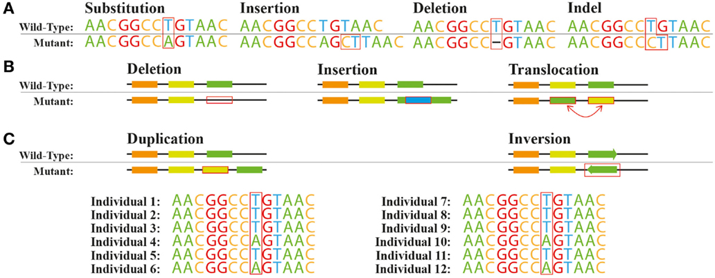
Beyond SNPs: Encoding Different Variant Types#
While we commonly encode SNPs, there are other types of genetic variations where the same principles also apply:
Insertions and Deletions (Indels)
Small insertions or deletions in DNA sequence
Typically encoded using the same 0/1/2 scheme as SNPs
Copy Number Variations (CNVs)
Deletions or duplications of larger DNA segments
Can be encoded as actual copy number (0, 1, 2, 3, etc.)
Structural Variants
Inversions, translocations, and complex rearrangements
Often encoded as binary (presence/absence)
The choice of encoding scheme should reflect the biological hypothesis about how the variant affects the phenotype. For more information, refer to Figure 1 in Cardoso et al., 2015.